API
1. 概述
A software framework for massively parallel, block-structured adaptive mesh refinement (AMR) applications
主要是C++,带有fortran接口
支持 1D、2D 和 3D
支持体心,面心,节点数据结构
支持粒子模拟,用于拉格朗日粒子追踪及多相流模拟
支持复杂几何的浸入边界法(切割单元)表示
支持分层自适应结构网格上的双曲线、抛物线和椭圆型方程求解
基于 MPI+X 的混合并行化策略,其中 X 是用于多核架构的 OpenMP,对于包括 NVIDIA GPU 的架构为CUDA,包括 AMD GPU 架构的为 HIP
2. 基础
2.1 数据结构
IntVect与IndexTypeIntVect为无量纲整数数组容器,其维度由AMREX_SPACEDIM决定,常作为索引数组IntVect iv(AMREX_D_DECL(127,127,127)); IntVect coarsening_ratio(AMREX_D_DECL(2,2,2)); iv.coarsen(2); // 每个元素除以2 iv.coarsen(coarsening_ratio); // 同上 const auto& iv2 = amrex::coarsen(iv, 2); // 返回一个IntVect同时修改iv IntVect iv3 = amrex::coarsen(iv, coarsening_ratio); // iv 不被修改
其中,宏
AMREX_D_DECL根据定义的维数展开成127或127,127或127,127,127IndexType定义了索引类型是体心还是节点,默认为全体心// Node in x-direction and cell based in y and z-directions IndexType xface(IntVect{AMREX_D_DECL(1,0,0)});
BoxBox为索引空间的抽象结构,包含一个IndexType和两个IntVect,分别表示矩形索引区域的上下角。通常定义方式为IntVect lo(AMREX_D_DECL(64,64,64)); IntVect hi(AMREX_D_DECL(127,127,127)); IndexType typ({AMREX_D_DECL(1,1,1)}); Box cc(lo,hi); // By default, Box is cell based. Box nd(lo,hi+1,typ); // Construct a nodal Box. Print() << "A cell-centered Box " << cc << "\n"; Print() << "An all nodal Box " << nd << "\n";
输出
A cell-centered Box ((64,64,64) (127,127,127) (0,0,0))
An all nodal Box    ((64,64,64) (128,128,128) (1,1,1))
BoxArray在给定加密等级下的Box集合
Box domain(IntVect{0,0,0}, IntVect{127,127,127});
BoxArray ba(domain);  // Make a new BoxArray out of a single Box
Print() << "BoxArray size is " << ba.size() << "\n";  // 1
ba.maxSize(64);       // Chop into boxes of 64^3 cells
Print() << ba;
输出
(BoxArray maxbox(8)
       m_ref->m_hash_sig(0)
((0,0,0) (63,63,63) (0,0,0)) ((64,0,0) (127,63,63) (0,0,0))
((0,64,0) (63,127,63) (0,0,0)) ((64,64,0) (127,127,63) (0,0,0))
((0,0,64) (63,63,127) (0,0,0)) ((64,0,64) (127,63,127) (0,0,0))
((0,64,64) (63,127,127) (0,0,0)) ((64,64,64) (127,127,127) (0,0,0)) )
FArrayBox定义在
Box上的数据(double, integer, complex, etc.)Box box(IntVect{0,0,0}, IntVect{63,63,63}); int ncomp = 2; FArrayBox fab1(box, ncomp); FArrayBox fab2(box, ncomp); fab1.setVal(1.0); // Fill fab1 with 1.0 fab1.mult(10.0, 0); // Multiply component 0 by 10.0 fab2.setVal(2.0); // Fill fab2 with 2.0 Real a = 3.0; // scalar alpha X plus Y fab2.saxpy(a, fab1); // For both components, fab2 <- a * fab1 + fab2
MultiFAB同一加密等级下
FArrayBox的集合包含定义每个FAB所属MPI进程的
DistributionMapping,默认使用空间填充曲线算法进行分配,在输入参数中可以自定义策略,如使用KNAPSACK负载均衡算法AMReX数据操作的主要单元
// ba is BoxArray
// dm is DistributionMapping
int ncomp = 4;
int ngrow = 1;
MultiFab mf(ba, dm, ncomp, ngrow);
这里定义
MultiFAB中有四个元素和一个ghost cell,意味着所包含的Box都增长1个网格数,即如果一个BoxArray中有Box{(7,7,7) (15 15 15)},则用来构建FArrayBox的会是Box{(6,6,6) (16,16,16)}。Ghost cells使得我们可以进行边界的stencil操作,有三种基本的边界类型:
内部边界
疏密网格交界边界
物理边界
自定义边界条件需要创建
BCRec对象,并对域的lo/hi边分别进行定义:Vector<BCRec> bc(phi.nComp()); for (int n = 0; n < phi.nComp(); ++n) { for (int idim = 0; idim < AMREX_SPACEDIM; ++idim) { if (geom.isPeriodic(idim)) { bc[n].setLo(idim, BCType::int_dir); // interior bc[n].setHi(idim, BCType::int_dir); } else { bc[n].setLo(idim, BCType::foextrap); // first-order extrapolation bc[n].setHi(idim, BCType::foextrap); } } }
这里用到了
amrex::BCType提供的基本边界条件:INT_DIR : 内部边界,包含周期边界,数据来自于其他网格或者插值
EXT_DIR : 外部迪利克雷边界,定义了边界上的值,需要自己写定义方式
HOEXTRAP : 边界处值来自于内部的高阶外推
FOEXTRAP : 边界处值来自于内部的一阶外推
REFLECT_EVEN : 反射边界 \(q(-i) = q(i)\)
REFLECT_ODD : 反射边界 \(q(-i)=-q(i)\)
下面给出常用物理边界的实施方式:
---------------------------------------------------------------------
          CONVERSIONS FROM PHYSICAL TO MATHEMATICAL BCs


PHYS BC        |   Velocity      |    Temperature   |    Scalars     |
----------------------------------------------------------------------
INTERIOR       |                 |                  |                |
   or          |    INT_DIR      |     INT_DIR      |    INT_DIR     |
PERIODIC       |                 |                  |                |
----------------------------------------------------------------------
               |                 |                  |                |
INFLOW         |    EXT_DIR      |     EXT_DIR      |    EXT_DIR     |
               |                 |                  |                |
----------------------------------------------------------------------
               |                 |                  |                |
OUTFLOW        |    FOEXTRAP     |     FOEXTRAP     |    FOEXTRAP    |
               |                 |                  |                |
----------------------------------------------------------------------
NO SLIP WALL   |                 |                  |                |
  with         |    EXT_DIR      |  REFLECT_EVEN    |    HOEXTRAP    |
ADIABATIC TEMP |    U = V = 0    |    dT/dn = 0     |                |
----------------------------------------------------------------------
NO SLIP WALL   |                 |                  |                |
  with         |    EXT_DIR      |     EXT_DIR      |    HOEXTRAP    |
FIXED TEMP     |    U = V = 0    |                  |                |
----------------------------------------------------------------------
SLIP WALL      |                 |                  |                |
  with         |  Un=0 EXT_DIR   |  REFLECT_EVEN    |    HOEXTRAP    |
ADIABATIC TEMP |  Ut   HOEXTRAP  |    dT/dn = 0     |                |
----------------------------------------------------------------------
SLIP WALL      |                 |                  |                |
  with         |  Un=0 EXT_DIR   |     EXT_DIR      |    HOEXTRAP    |
FIXED TEMP     |  Ut   HOEXTRAP  |                  |                |
----------------------------------------------------------------------
               |                 |                  |                |
SYMMETRY       |  Un REFLECT_ODD |  REFLECT_EVEN    | REFLECT_EVEN   |
               |  Ut REFLECT_EVEN|                  |                |
----------------------------------------------------------------------
2.2 循环和ParallelFor
使用迭代器MFIter进行循环操作
for (MFIter mfi(mf); mfi.isValid(); ++mfi) // 遍历网格
{
    // 当前FArrayBox下的“实”Box.
    // "实"是指BoxArray中不包含ghost cells的Box.
    const Box& box = mfi.validbox();

    // 当前FArrayBox的引用.
    FArrayBox& fab = mf[mfi];

    // 从FArrayBOox获取 Array4. 以便进行数组操作
    // 等价于  Array4<Real> const& a = mf.array(mfi);
    Array4<Real> const& a = fab.array();

    // 在指定的box上调用函数f1
    // 注意f1的作用不包含对ghost cell的操作
    f1(box, a);
}
// f1 示例
void f1 (Box const& bx, Array4<Real> const& a)
{
   const auto lo = lbound(bx);
   const auto hi = ubound(bx);
   for     (int k = lo.z; k <= hi.z; ++k) {
     for   (int j = lo.y; j <= hi.y; ++j) {
       for (int i = lo.x; i <= hi.x; ++i) {
         a(i,j,k) = ...
       }
     }
   }
}
MFIter只对其拥有的MPI进程下的网格进行循环,例如,进程0拥有2个Box,进程1拥有3个Box,则相应的MFIter迭代数为2和3。
AMReX提供循环的函数模板,以进行MPI或CUDA的并行计算
for (MFIter mfi(mfa,TilingIfNotGPU()); mfi.isValid(); ++mfi)
{
	const Box& bx = mfi.tilebox();
	Array4<Real> const& a = mfa[mfi].array();
	Array4<Real const> const& b = mfb[mfi].const_array();
	Array4<Real const> const& c = mfc[mfi].const_array();
	ParallelFor(bx, [=] AMREX_GPU_DEVICE (int i, int j, int k)
	{
		a(i,j,k) += b(i,j,k) * c(i,j,k);
	});
}
ParallelFor需要两个参数,首先是指定循环范围的Box,其次是一个自动推导的Lambda表达式使得循环在(i,j,k)网格上进行。上面的代码编译时无论是否使用GPU支持都可以运行,在有GPU支持时,AMREX_GPU_DEVICE指定了这是一个Device函数,将自动在GPU上实现并行。
2.3 示例
2.3.1 Hello World!
void test_Fab()
{
    int max_grid_size = 10;
    // 定义domain的上下边界
    amrex::IntVect dom_lo(AMREX_D_DECL(0, 0, 0));
    amrex::IntVect dom_hi(AMREX_D_DECL(19, 19, 19));
    amrex::Box domain(dom_lo, dom_hi);
	// 创建BoxArray
    amrex::BoxArray ba;
    ba.define(domain);
    // 切分为8个Box
    ba.maxSize(max_grid_size);
    // 物理边界坐标
    amrex::RealBox realbox({AMREX_D_DECL(0, 0, 0)}, {AMREX_D_DECL(1, 1, 1)});
    amrex::Geometry geo;
    // 定义domain在三个维度上都是周期性边界
    amrex::Array<int, AMREX_SPACEDIM> is_periodic{AMREX_D_DECL(1, 1, 1)};
    geo.define(domain, realbox, amrex::CoordSys::cartesian, is_periodic);
    // GpuArray可以是Host或Device函数,在不使用GPU支持时就相当于普通Array(Host变量)
    amrex::GpuArray<amrex::Real, AMREX_SPACEDIM> dx = geo.CellSizeArray();
	// ghost cell数以及分量数
    int Nghost = 1;
    int Ncomp = 1;
    amrex::DistributionMapping dm(ba);
    // 创建只有一个分量的MultiFab
    amrex::MultiFab phi(ba, dm, Ncomp, Nghost);
	// 统计MFIter循环次数,supposed to be 8
    int count = 0;
    for (amrex::MFIter mfi(phi); mfi.isValid(); ++mfi)
    {
        const amrex::Box &bx = mfi.validbox();
		// 创建对于MultiFab数据的引用
        const amrex::Array4<amrex::Real> &phiOld = phi.array(mfi);

        // set phi = 1 + e^(-(r-0.5)^2)
        amrex::ParallelFor(bx, [=] AMREX_GPU_DEVICE(int i, int j, int k) {
            // cell centered data here
            amrex::Real x = (i + 0.5) * dx[0];
            amrex::Real y = (j + 0.5) * dx[1];
            amrex::Real z = (k + 0.5) * dx[2];
            amrex::Real rsquared = ((x - 0.5) * (x - 0.5) + (y - 0.5) * (y - 0.5) + (z - 0.5) * (z - 0.5)) / 0.01;
            phiOld(i, j, k) = 1. + std::exp(-rsquared);
        });
        count += 1;
    }
    const int IOProc = amrex::ParallelDescriptor::IOProcessorNumber();
    // 得到所有进程下count的和
    amrex::ParallelDescriptor::ReduceIntSum(count, IOProc);
    amrex::Print() << count << std::endl;
    // std::string amrex::Concatenate(const std::string &root, int num, int mindigits = 5)
    const std::string &pltfile = amrex::Concatenate("plt", 0, 5);
    amrex::WriteSingleLevelPlotfile(pltfile, phi, {"phi"}, geo, 0, 0);
}
sdp@ENIAC:~$ mpirun -n 3 ./_home_sdp_Tutorials_Basic_main_C
MPI initialized with 3 MPI processes
MPI initialized with thread support level 0
AMReX (21.10-8-g64c9d92c0f46) initialized
8
AMReX (21.10-8-g64c9d92c0f46) finalized
3. 自适应块结构网格
3.1 特点
在感兴趣的区域加密网格
在每一个patch上是结构化的,保持高差分精度,离散化和数据获取都很简单
自然地支持分层并行
只需要在粗细网格交界处采用特殊的离散方式
3.2 Patch-Based vs OctTree
组织加密层级的两种不同的数据结构,AMReX采用Patch-Based而OpenFOAM采用八叉树结构
3.3 时间推进策略
为了使得不同层级间的数据推进到同一时间,可以采用两种时间推进策略:subcycling or non-subcycling
Non-subcycling:
在所有加密等级上采用同一 \(dt\),同步推进
Subcycling:
在细网格使用较小的\(dt\),粗网格上使用较大的\(dt\),网格间需要进行同步以确保守恒性
考虑一个两层网格的二维模拟,标准的时间推进策略是:首先不考虑细网格,在粗网格上进行时间推进,然后将粗网格上的值作为边界条件进行细网格的时间推进。但是这将造成粗细网格交界处,粗网格上的通量通常不等于细网格上的通量,造成全局的不守恒。在sub-cycle策略中,如果采用\(r\)的网格加密比,则在细网格上采用\(dt/r\)的时间步长,进行\(r\)次时间推进,然后再使用通量寄存器FluxRegiser进行修正。
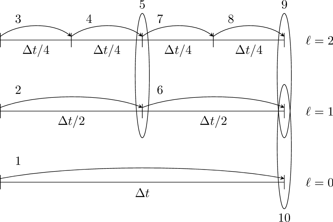
例如,一个三层的模拟,采用递归方式进行时间推进和通量同步。
标量输运
使用
求解\(\phi(x,y,t)\)。其中速度场\(\boldsymbol{u}^{spec} = (u,v)\)是给定的无旋场。由下式给出
理论上来讲,速度场是周期性的无旋场,控制方程中也不包含粘性耗散项,因此经过一个周期后,\(\phi\)的分布应该与初始分布相同。由于数值误差和耗散的存在,实际不完全相同。
采用离散
其中\(\phi\)定义在体心上,\(\boldsymbol{u}\)定义在面上,为了计算得到面通量,面上的\(\phi\)值通过Godunov格式得到。

可以计算得到在最粗网格上的\(t=0\)与\(t=2\)时刻\(\phi\)的差
            variable name            absolute error            relative error
                                        (||A - B||)         (||A - B||/||A||)
 ----------------------------------------------------------------------------
 level = 0
 phi                                  0.01563385663            0.007879356458
4. 其他特性
4.1 与pyTorch耦合的机器学习
AMReX 和 LibTorch 可以使用 GCC 编译器在相同的环境中编译。数据在 AMReX 中使用称为multifab的结构表示。为了在 AMReX 上调用预先训练好的机器学习模型,需要将数据从multifab转换为 Torch 张量。